GPSANS Data Process Guide

Quick Reference for using jupyter notebook to reduce data

Note:

• This is a quick reference to guide you through using data reduction for GP-SANS. It will not replace the function of your instrument local contact, who is the primary resource for the instrument related questions. Please work with her/him to setup and understand the data reduction process before using the guide.

• Various on-line systems will be used for this process, you should have your ORNL GUEST Portal login and password handy. They are accessible both inside and outside ORNL.

  • Data catalog https://oncat.ornl.gov (Demo )

  • Data reduction notebook script interface https://jupyter.sns.gov

  • Data analysis cluster, where all data are located https://analysis.sns.gov/

• A companion video tutorial can be found in YouTube: GP-SANS tutorials (1config and multi_config)

1. Identify the run numbers for the data in ONCat.ornl.gov : All data are saved in sequential number (Run #) with all metadata information such as title, time and other user specified information. The run number is used in the reduction to call the data. Identifying the run number for the data to be reduced in the data catalog is the first step in the process.

   1. Login into oncat.ornl.gov
      

   2. Click into HFIR > CG2, then find your experiment IPTS and click on the blue button. This will take you to the runs tab.

   3. The Run number is the very first column in the list, along with other useful information to identify data as seen in figure below.

   4. You can click "download CSV" in the upper right corner of the runs tab to get a tab delimited list of your data along with pertinent metadata.

   5. The table below is a good way of organizing run data for samples and configurations on GP-SANS. Use the run numbers and information from OnCat to populate table for your experiment with local contact's help. This table will help you fill out the different sections of the juypter notebook for data reduction.

|-----------+----------+----------+----------+----------+----------| | Sample
  | 19m12A
scatt+trans | 8m4.75A
scatt | 8m4.75A
trans | 2m4.75A
scatt | 2m4.75A
center | |===========+==========+==========+==========+==========+==========| | Porasil B | 10597 | 10605 | 10613 | 10621 | 10634 | |-----------+----------+----------+----------+----------+----------| | Ag Beh | 10598 | 10606 | 10614 | 10622 | | |-----------+----------+----------+----------+----------+----------| | H20 | 10599 | 10607 | 10615 | 10623 | | |-----------+----------+----------+----------+----------+----------| | Al4 | 10600 | 10608 | 10616 | 10624 | | |-----------+----------+----------+----------+----------+----------| | D20 | 10601 | 10609 | 10617 | 10625 | | |-----------+----------+----------+----------+----------+----------| | MT cell | 10602 | 10610 | 10618 | 10626 | | |-----------+----------+----------+----------+----------+----------| | Mt air | 10637 | 10638 | 10639 | 10640 | 10641 | |===========+==========+==========+==========+==========+==========| | | sample_ | sample_ | sample_ | sample_ | bc_ | | | config_1 | config_2 | config_2 | config_3 | config_3 | |-----------+----------+----------+----------+----------+----------|

{:start="2"} 2. Data reduction with jupyter notebook, jupyter.sns.gov

1.  Log into jupyter.sns.gov.

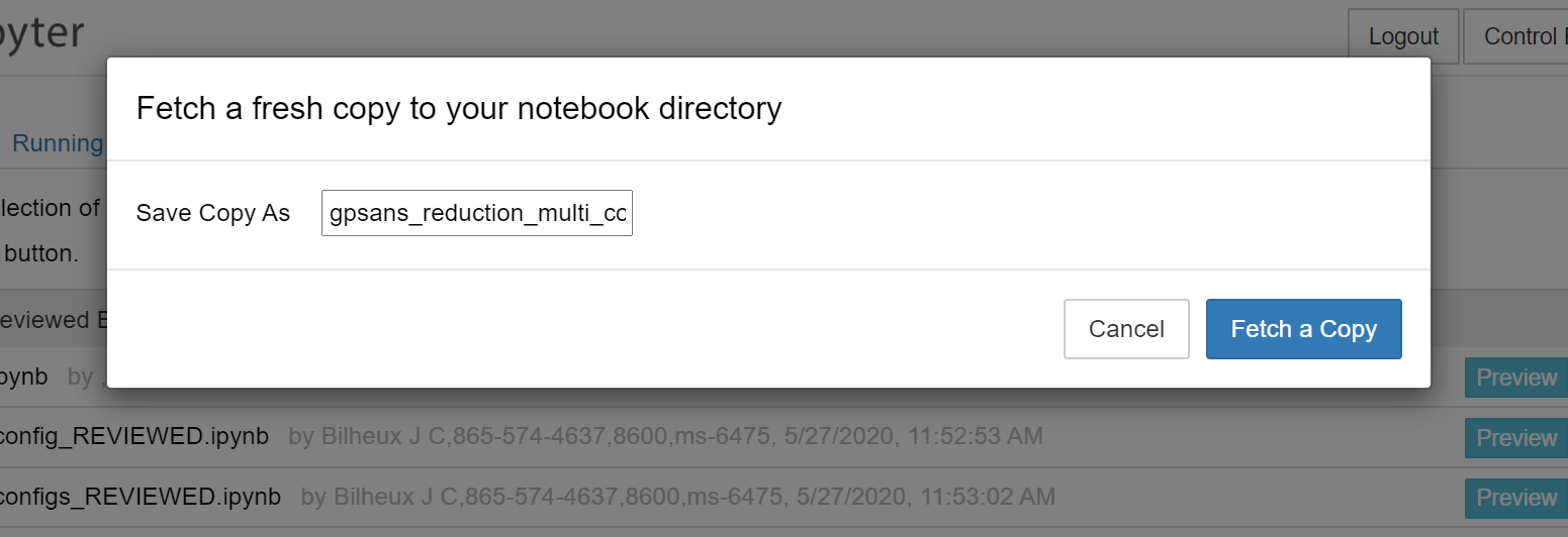
2.  Your local contact will direct you to the best example for your
experiment. These examples can be found on the examples tab. For
this guide use
gpsans_reduction_multi_config.ipynb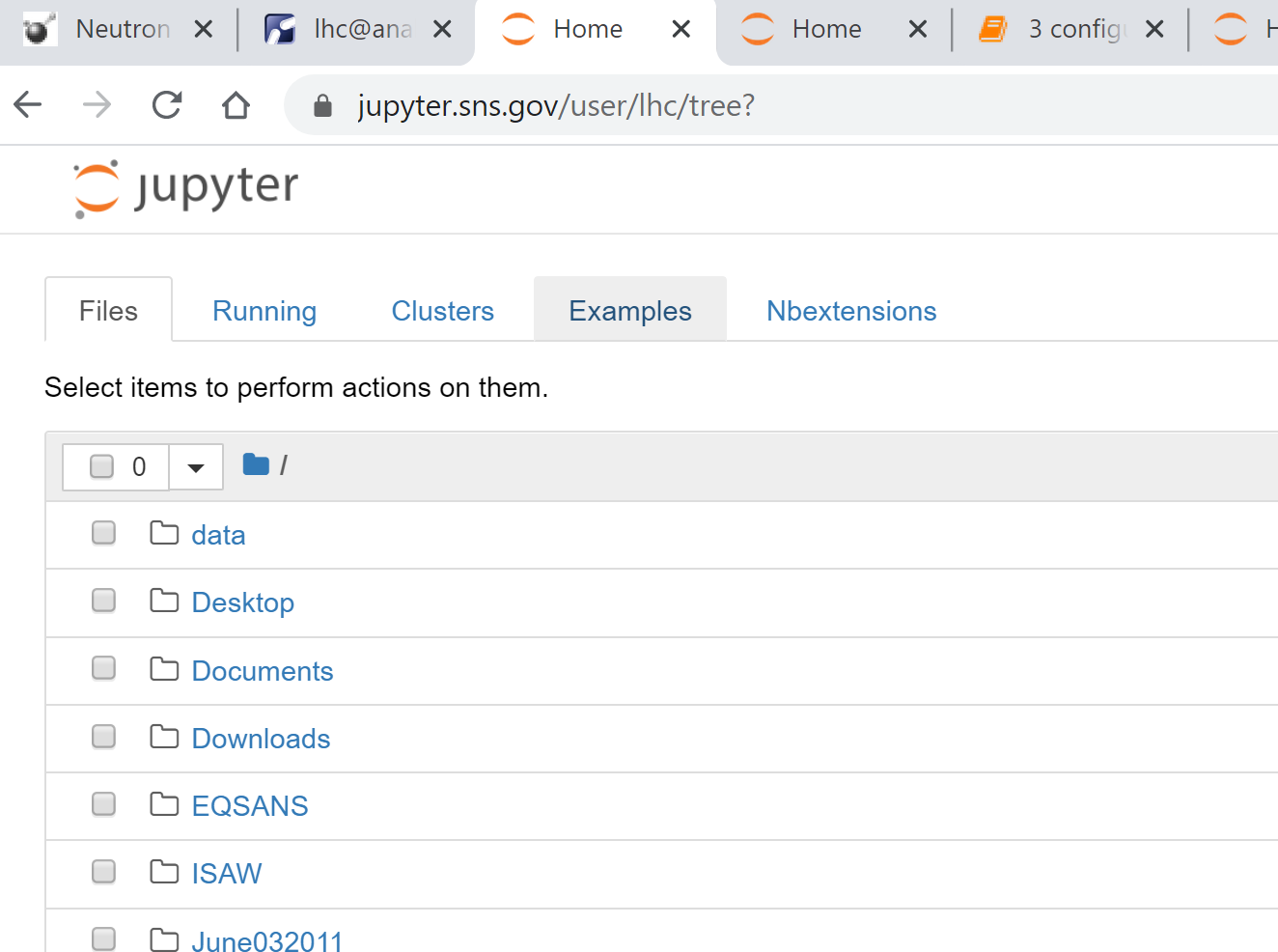![](images/gpsans_image6.png)

3.  Click "Use" and fetch a copy to your home directory on the analysis
cluster.
![](images/gpsans_image7.png)

4.  The first cell is for setting up your data. This is where the table
you created in 1.5 will come in handy.
![](images/gpsans_image8.png)

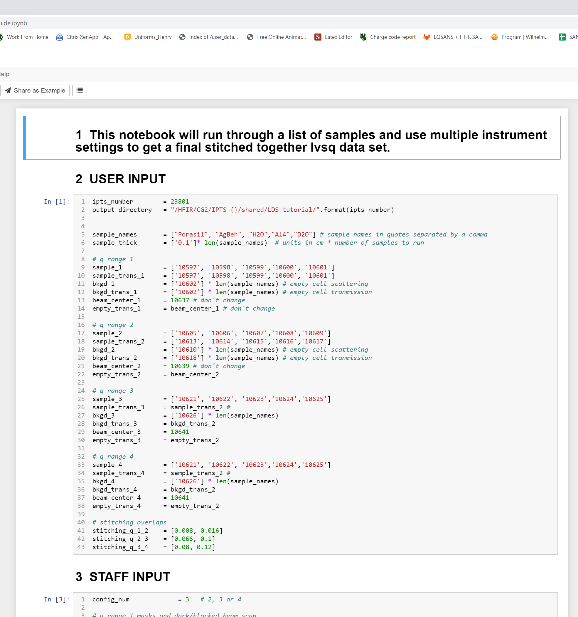
**Sample_names**: the reduced data will be saved with the text as prefix

***Samples_config_1***: run numbers for the data to be reduced,
multiple run numbers can be use with comma (,) or dash (-, a range of
run numbers) for a specific configuration.

*Samples_config_2, samples_config_3 and samp*les_config_4 are for the
run numbers for the other configurations in your run table.

*Bkg_1*: run numbers for the background to be subtracted for a
specific configuration.

*Bkgd_config_2,Bkgd_config_3,Bkgd_config_4* are the backgrounds for the
other configurations in your run table

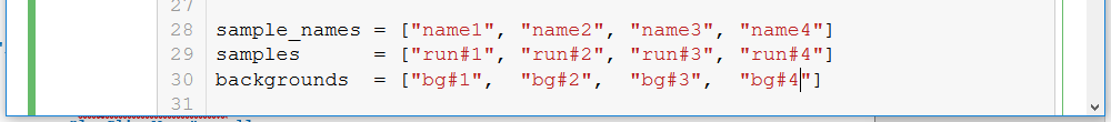
The number of items in the multiple configurations lists must be the
same as they are in one-to-one correspondence during the reduction
loop.

For example:
![](images/gpsans_image9.png)
**Note:**
 -   Sometimes for the lowest q setting, the scattering and transmission
 will be the same data file. Please use the same list for example:
 sample_config_1 and sample_trans_config_1.

 -   For the config_3, the transmission usually but not always comes from
 config_2 as long as the wavelength, collimation, and sample aperture
 remains the same between configurations.

 -   The merging and scaling process are handled by the reduction
 process.

{:start="5"}
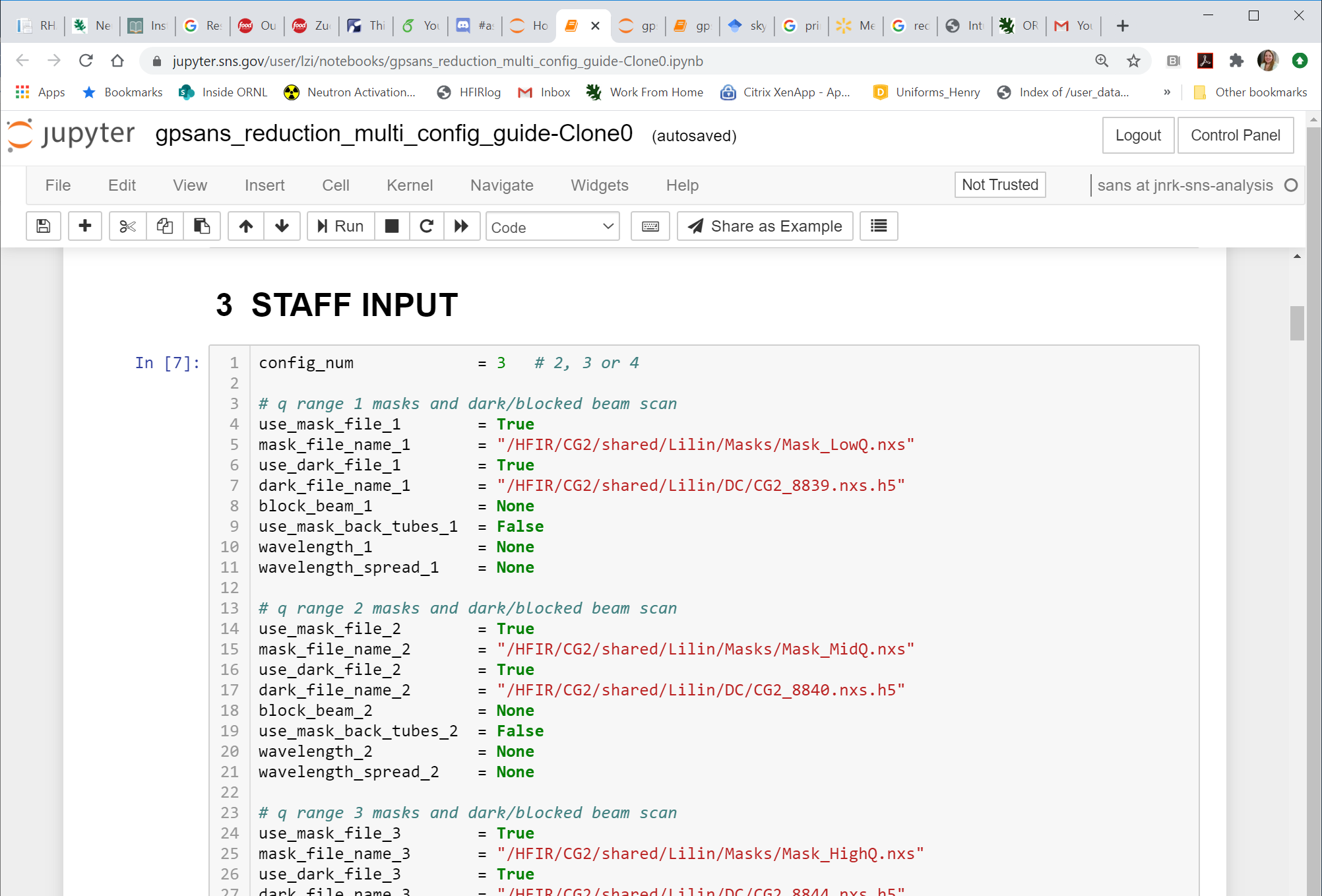
5.  The second cell labeled "Staff Input" will be filled out by your
local contact and contain specific settings for the instrument,
i.e. detector sensitivity correction. Once the run numbers are
inputted and the local contact has filled out the staff section,
click the Run button at the top of the page to run the entire
notebook. Another way to run the notebook is to hit ctrl+Enter
in each cell to run them individually.
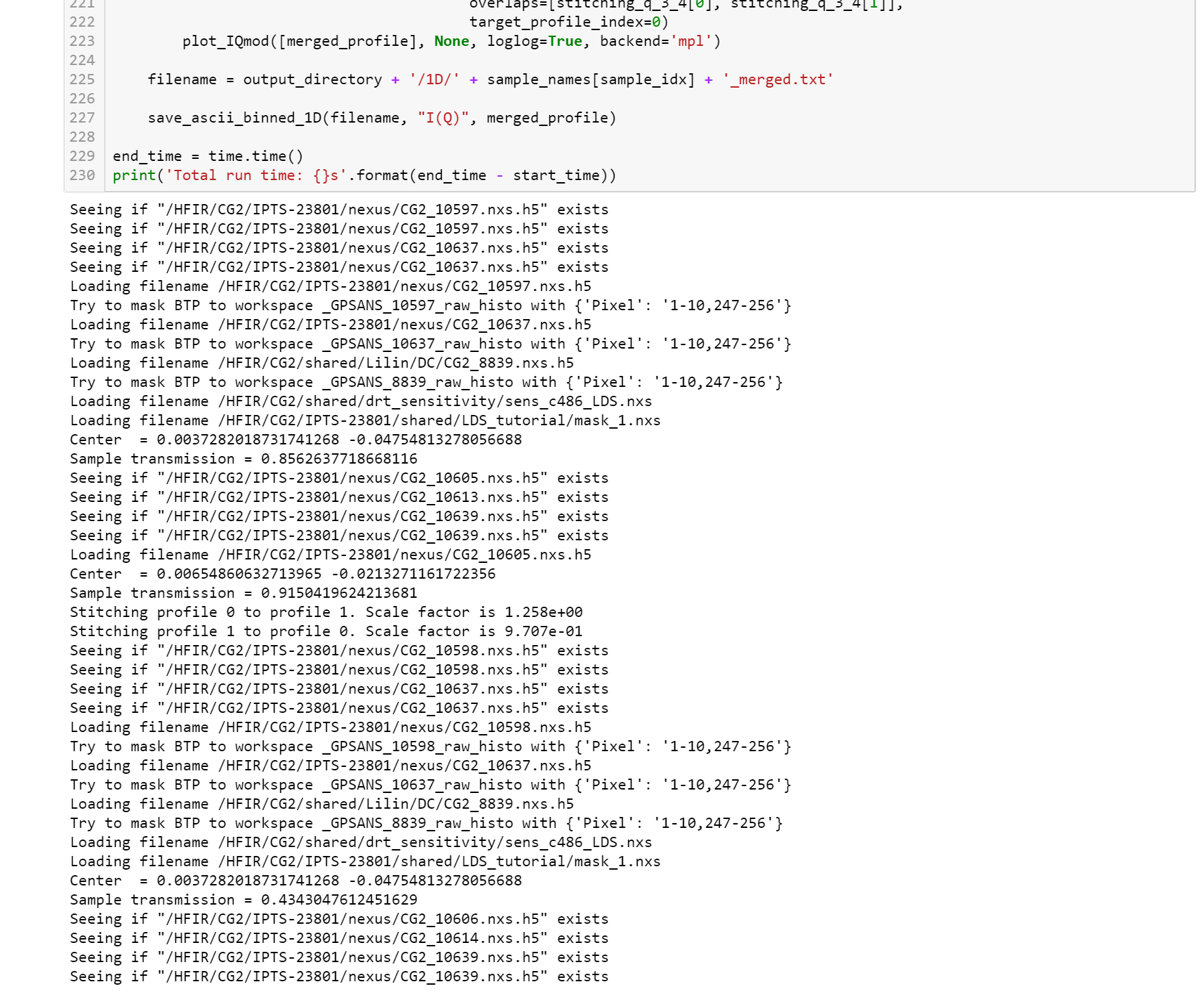
![](images/gpsans_image10.png)The
data will be reduced in the order of the list. Some useful information
will be displayed, e.g., the progress, the transmissions etc. The
information is also saved into a reduction_log.hdf5 file that will
appear in the output directory you specified in User Input section.
![](images/gpsans_image11.png)

3. Download and view the data from analysis.sns.gov

The reduced data and metadata are all saved in the folder designated by users on analysis.sns.gov. The server provides various connection options to download the data, with support from linux@support.sns.gov. Here, we will show you how to locate the folder and files with the Remote Desktop, which can be launched from any browser by click "Launch Session"

1. Once logged in, it is a full functional remote desktop. You can use the file broswer to locate the files reduced.

2. Reduced files are saved into 1D folder (1D curves) and 2D folder (reduced in Qx-Qy plane). The HDF files have all the raw and reduction meta data, as well as the reduced data. Please consult your local contact on how to utilize them.

   

3. The typical isotropic data in 1D format are saved in the 1D folder with merged data if multiple configurations are used. They are typical SANS data format of 4 columns: Q, I, ΔI, ΔQ. You can download them and view them in the SANS analysis software of your choice.

Up: Index